Modeling With Continuous Variables in Sas
1. A standard ANOVA
2. A standard ANCOVA
3. Estimate slopes for each diet group
4. Test equality of slopes across diet groups
5. Perform tests with separate slopes for all diet groups
5.1 Comparing diet 1 with diet 2
5.2 Comparing diets 1 and 2 to the control group
6. Testing to pool slopes
7. Perform tests with some pooled slopes
7.1 Overall analysis pooling slopes for diet groups 2 and 3
7.2 Comparing diet groups 1 and 2 when pooling slopes for diet groups 2 and 3
7.3 Comparing diet groups 2 and 3 when pooling slopes for diet groups 2 and 3
8. Summary
Analysis of covariance (ANCOVA) is a statistical procedure that allows you to include both categorical and continuous variables in a single model. ANCOVA assumes that the regression coefficients are homogeneous (the same) across the categorical variable. Violation of this assumption can lead to incorrect conclusions. This page will explore what happens when you have heterogeneous (different) regressions across groups and show some strategies for dealing with them. This involves some complex topics in the use of proc glm, especially the estimate statement.
Here is an example data file we will use. It contains 30 subjects who used one of three diets, diet 1 (diet=1), diet 2 (diet=2) and a control group (diet=3). Before the start of the study, the height of the subject was measured, and after the study the weight of the subject was measured.
DATA htwt; INPUT id diet height weight ; CARDS; 1 1 56 140 2 1 60 155 3 1 64 143 4 1 68 161 5 1 72 139 6 1 54 159 7 1 62 138 8 1 65 121 9 1 65 161 10 1 70 145 11 2 56 117 12 2 60 125 13 2 64 133 14 2 68 141 15 2 72 149 16 2 54 109 17 2 62 128 18 2 65 131 19 2 65 131 20 2 70 145 21 3 54 211 22 3 58 223 23 3 62 235 24 3 66 247 25 3 70 259 26 3 52 201 27 3 59 228 28 3 64 245 29 3 65 241 30 3 72 269 ; RUN;
1. A standard ANOVA
You could analyze this data with a standard ANOVA, as shown below. This analysis compares the weights of the three groups. It also uses the contrast statement to compare the two diets (1 and 2) to the control group (diet 3). We also want to compare diet 1 with diet 2.
PROC GLM DATA=htwt; CLASS diet ; MODEL weight = diet ; MEANS diet / deponly ; CONTRAST 'compare 1&2 with control' diet 1 1 -2 ; CONTRAST 'compare diet 1 with 2 ' diet 1 -1 0 ; RUN; QUIT;General Linear Models Procedure Class Level InformationClass Levels Values
DIET 3 1 2 3
Number of observations in data set = 30
General Linear Models Procedure
Dependent Variable: WEIGHT Sum of Mean Source DF Squares Square F Value Pr > F
Model 2 64350.600000 32175.300000 128.48 0.0001
Error 27 6761.400000 250.422222
Corrected Total 29 71112.000000
R-Square C.V. Root MSE WEIGHT Mean
0.904919 9.254231 15.824735 171.00000
Source DF Type I SS Mean Square F Value Pr > F
DIET 2 64350.600000 32175.300000 128.48 0.0001
Source DF Type III SS Mean Square F Value Pr > F
DIET 2 64350.600000 32175.300000 128.48 0.0001
General Linear Models Procedure
Level of ————WEIGHT———– DIET N Mean SD
1 10 146.200000 12.8391762 2 10 130.900000 12.2424580 3 10 235.900000 20.8936460 General Linear Models Procedure
Dependent Variable: WEIGHT
Contrast DF Contrast SS Mean Square F Value Pr > F
compare 1&2 with con 1 63180.150000 63180.150000 252.29 0.0001 compare diet 1 with 1 1170.450000 1170.450000 4.67 0.0397
The ANOVA results show an overall difference among all of the diets and the contrasts show a difference between the control group and the two diets, and a difference between diet 1 and diet 2. The ANOVA disregards the information that we have about the subject's height. As height is probably correlated with weight, this could be useful as a covariate in an ANCOVA.
2. A standard ANCOVA
Below we perform a standard ANCOVA.
PROC GLM DATA=htwt; CLASS diet ; MODEL weight = diet height / SOLUTION ; LSMEANS diet ; CONTRAST 'compare control with 1,2' diet 1 1 -2 ; CONTRAST 'compare 1 with 2 ' diet 1 -1 0 ; RUN; QUIT;
The results are consistent with those of the ANOVA. There is an overall effect of diet. Also, the control group is significantly different from the two diets, and diet 1 is different from diet 2. The significance level for the comparison of diet 1 versus diet 2 is smaller than the standard ANOVA.
General Linear Models Procedure Class Level Information
Class Levels Values
DIET 3 1 2 3
Number of observations in data set = 30 General Linear Models Procedure
Dependent Variable: WEIGHT Sum of Mean Source DF Squares Square F Value Pr > F
Model 3 67409.811075 22469.937025 157.80 0.0001
Error 26 3702.188925 142.391882
Corrected Total 29 71112.000000
R-Square C.V. Root MSE WEIGHT Mean
0.947939 6.978250 11.932807 171.00000
Source DF Type I SS Mean Square F Value Pr > F
DIET 2 64350.600000 32175.300000 225.96 0.0001 HEIGHT 1 3059.211075 3059.211075 21.48 0.0001
Source DF Type III SS Mean Square F Value Pr > F
DIET 2 66726.086524 33363.043262 234.30 0.0001 HEIGHT 1 3059.211075 3059.211075 21.48 0.0001
T for H0: Pr > |T| Std Error of Parameter Estimate Parameter=0 Estimate
INTERCEPT 126.1382736 B 5.26 0.0001 23.97915732 DIET 1 -92.1705212 B -17.19 0.0001 5.36306483 2 -107.4705212 B -20.04 0.0001 5.36306483 3 0.0000000 B . . . HEIGHT 1.7646580 4.64 0.0001 0.38071364
NOTE: The X'X matrix has been found to be singular and a generalized inverse was used to solve the normal equations. Estimates followed by the letter 'B' are biased, and are not unique estimators of the parameters.
General Linear Models Procedure Least Squares Means
DIET WEIGHT LSMEAN
1 145.376493 2 130.076493 3 237.547014
General Linear Models Procedure
Dependent Variable: WEIGHT
Contrast DF Contrast SS Mean Square F Value Pr > F
compare control with 1 65555.636524 65555.636524 460.39 0.0001 compare 1 with 2 1 1170.450000 1170.450000 8.22 0.0081
Because we used the solution option, we are shown the regression coefficients and see the coefficient (slope) between height and weight is 1.76. Figure 1 below shows the scatterplot between height and weight and the line of best fit with slope 1.76.
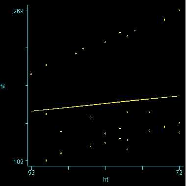
Figure 1. Scatterplot of weight by height with overall regression line
3. Estimate slopes for each diet group
One assumption of ANCOVA is that the slope between height and weight is the same for the three diet groups. This is called the homogeneity of regression assumption. Below we show a scatterplot like the one above; however, this one shows the three diet groups in different colors and shows a separate regression line for each diet group (diet 1=blue, diet 2=yellow, diet 3=red). As you can see the blue regression line looks like it has a very different slope from the other two regression lines.
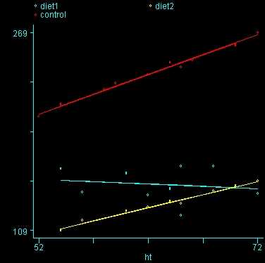
Figure 2. Scatterplot of weight by height with separate regression lines for each group (diet 1=blue, diet 2=yellow, diet 3=red)
Below we perform an analysis that shows the slopes of each of the lines. Even if we found the slope between height and weight to be 0 in the prior analysis, this is still a useful analysis to perform. It is possible that the overall slope for the entire sample was 0, but the slopes for some groups were positive and the others were negative and they cancelled each other out. This analysis would help you see if such a pattern was occurring.
PROC SORT DATA=htwt; BY diet; RUN; PROC GLM DATA=htwt; BY diet ; MODEL weight = height / SOLUTION ; RUN; QUIT;
We indeed see below that the slopes seem very different. (Note that the output has been abbreviated.) The slope for diet 1 (-.37) is much smaller than the slope for diet 2 (2.095) and the control group, diet=3 (3.189). We need to check into this further and test whether these slopes are significantly different from each other.
diet=1 Dependent Variable: weight Standard Parameter Estimate Error t Value Pr > |t| Intercept 170.1664447 49.43018216 3.44 0.0088 height -0.3768309 0.77433413 -0.49 0.6396 diet=2 Dependent Variable: weight Standard Parameter Estimate Error t Value Pr > |t| Intercept -2.397470040 7.05327189 -0.34 0.7427 height 2.095872170 0.11049098 18.97 <.0001 diet=3 Dependent Variable: weight Standard Parameter Estimate Error t Value Pr > |t| Intercept 37.49895178 7.70303233 4.87 0.0012 height 3.18972746 0.12323669 25.88 <.0001
4. Test equality of slopes across diet groups
We can test to see if the slopes for the three diet groups are equal, as shown below. The diet*height effect tests if the three slopes are equal.
PROC GLM DATA=htwt; CLASS diet ; MODEL weight = diet height diet*height ; RUN; QUIT;
The diet*height effect is indeed significant, indicating that the slopes do differ across the three diet groups. (Note that we look at the Type III SS, consistent with our general recommendations to use Type III instead of Type I SS.) The output is abbreviated to save space.
<some output omitted> Source DF Type III SS Mean Square F Value Pr > F DIET 2 1224.0043440 612.0021720 9.68 0.0008 HEIGHT 1 2597.0189017 2597.0189017 41.10 0.0001 HEIGHT*DIET 2 2185.5435689 1092.7717845 17.29 0.0001
5. Perform tests with separate slopes for all diet groups
Because the slopes for the three diet groups are not the same, we should not use a traditional ANCOVA model that assumes the slopes for the three diet groups are the same. Instead, we can use a model that estimates separate slopes for all three diet groups. Because the diet groups will have different slopes, we must be very cautious in interpreting adjusted means. One way of thinking about this is to focus on the fact that we have a diet*height interaction. This means that we cannot interpret the relationship between height and weight without referring to diet. Likewise, if we want to talk about the effect of diet we need to specify what height we are talking about. For example, in comparing diets 1 and 2 (in Figure 2) it looks like there is no difference between diets 1 and 2 (blue and yellow) for tall people, but there may be a difference for shorter people. Below, we will see how to make these comparisons.
5.1 Comparing diet 1 with diet 2
Let us compare diet 1 versus diet 2 at three different levels of height, for those who are 59 inches tall, 64 inches and 68 inches tall. These correspond to the 25th, 50th and 75th percentiles for height. We can then evaluate separately for each height group the difference between diet 1 and diet 2.
The model used in this analysis is the same as the model from section 4 where we estimated separate slopes. In addition we use the estimate statement for comparing the diets 1 and 2 at the three levels of height, and for obtaining the adjusted mean for weight.
The first three estimate statements compare diet 1 with diet 2 at 59, 64, and 68 inches. The next three estimate statements request the predicted value of weight for people on diet 1 who are 59 inches, 64 inches, and 68 inches tall. The next three estimate statements requests the weight for people on diet 2 who are 59 inches, 64 inches, and 68 inches tall.
PROC GLM DATA=htwt; CLASS diet ; MODEL weight = diet height diet*height ; ESTIMATE 'diet 1 vs 2 at 59 in' diet -1 1 0 diet*height -59 59 0 ; ESTIMATE 'diet 1 vs 2 at 64 in' diet -1 1 0 diet*height -64 64 0 ; ESTIMATE 'diet 1 vs 2 at 68 in' diet -1 1 0 diet*height -68 68 0 ; ESTIMATE 'wt for diet 1 at 59 in' intercept 1 diet 1 0 0 height 59 diet*height 59 0 0 ; ESTIMATE 'wt for diet 1 at 64 in' intercept 1 diet 1 0 0 height 64 diet*height 64 0 0 ; ESTIMATE 'wt for diet 1 at 68 in' intercept 1 diet 1 0 0 height 68 diet*height 68 0 0 ; ESTIMATE 'wt for diet 2 at 59 in' intercept 1 diet 0 1 0 height 59 diet*height 0 59 0 ; ESTIMATE 'wt for diet 2 at 64 in' intercept 1 diet 0 1 0 height 64 diet*height 0 64 0 ; ESTIMATE 'wt for diet 2 at 68 in' intercept 1 diet 0 1 0 height 68 diet*height 0 68 0 ; RUN; QUIT;
For the sake of saving space, we show just the output related to the estimate statements.
<output omitted to save space> Standard Parameter Estimate Error t Value Pr > |t| diet 1 vs 2 at 59 in -26.674434 4.64126551 -5.75 <.0001 diet 1 vs 2 at 64 in -14.310919 3.56455159 -4.01 0.0005 diet 1 vs 2 at 68 in -4.420107 4.55895082 -0.97 0.3419 wt for diet 1 at 59 in 147.933422 3.28187031 45.08 <.0001 wt for diet 1 at 64 in 146.049268 2.52051860 57.94 <.0001 wt for diet 1 at 68 in 144.541944 3.22366504 44.84 <.0001 wt for diet 2 at 59 in 121.258988 3.28187031 36.95 <.0001 wt for diet 2 at 64 in 131.738349 2.52051860 52.27 <.0001 wt for diet 2 at 68 in 140.121838 3.22366504 43.47 <.0001
Focusing on the comparison of diets 1 and 2, these results indicate a significant difference between diet 1 and diet 2 for those 59 inches tall (t=-5.75, p < .0001) and a significant difference for those 64 inches tall (t=-4.01, p=0.0005). For those who are tall (i.e., 68 inches), diet 1 and diet 2 are about equally effective. This corresponds with what we saw in Figure 2.
You will notice that if you take the parameter estimate for "wt for diet 1 at 59 in" minus the parameter estimate for "wt for diet 2 at 59 in", you get -26.67, which is the parameter estimate for "diet 1 vs. 2 at 59 in" (147.93 – 121.25 = -26.67). Likewise, taking the parameter estimate for "wt for diet 1 at 64 in" minus the parameter estimate for "wt for diet 2 at 64in" yields the parameter estimate for "diet 1 vs. 2 at 64 in" (146.04-131.73 = -14.31). You can do a similar computation for the weights for those 68 inches tall.
It can be very difficult to construct estimate statements, so here is a shortcut that works when you want to compare one group versus another group using the lsmeans statement.
PROC GLM DATA=htwt; CLASS diet ; MODEL weight = diet height diet*height ; LSMEANS diet / AT height=59 PDIFF ; LSMEANS diet / AT height=64 PDIFF ; LSMEANS diet / AT height=68 PDIFF ; RUN; QUIT;
For the sake of saving space, we show just the output related to the lsmeans statements. As you can see, the results comparing diet 1 and 2 are the same using lsmeans as using estimate. For example, for those 59 inches tall, the adjusted mean for diet 1 is 147.93 and the adjusted mean for diet 2 is 121.25, and this is significant with p<.0001 (see italics in output).
<some output omitted to save space> The GLM Procedure Least Squares Means at height=59 weight LSMEAN diet LSMEAN Number 1 147.933422 1 2 121.258988 2 3 225.692872 3 Least Squares Means for effect diet Pr > |t| for H0: LSMean(i)=LSMean(j) Dependent Variable: weight i/j 1 2 3 1 <.0001 <.0001 2 <.0001 <.0001 3 <.0001 <.0001 NOTE: To ensure overall protection level, only probabilities associated with pre-planned comparisons should be used. The GLM Procedure Least Squares Means at height=64 weight LSMEAN diet LSMEAN Number 1 146.049268 1 2 131.738349 2 3 241.641509 3 Least Squares Means for effect diet Pr > |t| for H0: LSMean(i)=LSMean(j) Dependent Variable: weight i/j 1 2 3 1 0.0005 <.0001 2 0.0005 <.0001 3 <.0001 <.0001 NOTE: To ensure overall protection level, only probabilities associated with pre-planned comparisons should be used. The GLM Procedure Least Squares Means at height=68 weight LSMEAN diet LSMEAN Number 1 144.541944 1 2 140.121838 2 3 254.400419 3 Least Squares Means for effect diet Pr > |t| for H0: LSMean(i)=LSMean(j) Dependent Variable: weight i/j 1 2 3 1 0.3419 <.0001 2 0.3419 <.0001 3 <.0001 <.0001 NOTE: To ensure overall protection level, only probabilities associated with pre-planned comparisons should be used.
It each much easier to use lsmeans for comparing groups than estimate, however lsmeans can only make pairwise comparisons. But we are also interested in comparing the two diets (diet 1 and diet 2) combined to the control group (diet 3). For that, we must use estimate since lsmeans will not do that kind of comparison, as shown below.
5.2 Comparing diets 1 and 2 to the control group
The analysis below compares diets 1 and 2 to the control group (group 3) at the three different heights: 59 inches, 64 inches and 68 inches. The first three estimate commands compare diets 1 and 2 to the control group at these three different heights. The next three estimate commands estimate the weight for the diet 1 and diet 2 groups combined at the three heights. The following estimate commands estimate the weight for the control group at the three heights.
PROC GLM DATA=htwt; CLASS diet ; MODEL weight = diet height diet*height ; ESTIMATE 'diet 1&2 vs 3 at 59in' diet .5 .5 -1 diet*height 29.5 29.5 -59 ; ESTIMATE 'diet 1&2 vs 3 at 64in' diet .5 .5 -1 diet*height 32 32 -64 ; ESTIMATE 'diet 1&2 vs 3 at 68in' diet .5 .5 -1 diet*height 34 34 -68 ; ESTIMATE 'wt diet 1&2 at 59in' intercept 1 diet .5 .5 0 height 59 diet*height 29.5 29.5 0 ; ESTIMATE 'wt diet 1&2 at 64in' intercept 1 diet .5 .5 0 height 64 diet*height 32 32 0 ; ESTIMATE 'wt diet 1&2 at 68in' intercept 1 diet .5 .5 0 height 68 diet*height 34 34 0 ; ESTIMATE 'wt control at 59in' intercept 1 diet 0 0 1 height 59 diet*height 0 0 59 ; ESTIMATE 'wt control at 64in' intercept 1 diet 0 0 1 height 64 diet*height 0 0 64 ; ESTIMATE 'wt control at 68in' intercept 1 diet 0 0 1 height 68 diet*height 0 0 68 ; RUN; QUIT;
For the sake of saving space, we show just the output related to the estimate statements.
<some output omitted to save space> Standard Parameter Estimate Error t Value Pr > |t| diet 1&2 vs 3 at 59in -91.096667 3.66066279 -24.89 <.0001 diet 1&2 vs 3 at 64in -102.747701 3.16739826 -32.44 <.0001 diet 1&2 vs 3 at 68in -112.068528 4.13354574 -27.11 <.0001 wt diet 1&2 at 59in 134.596205 2.32063275 58.00 <.0001 wt diet 1&2 at 64in 138.893808 1.78227579 77.93 <.0001 wt diet 1&2 at 68in 142.331891 2.27947541 62.44 <.0001 wt control at 59in 225.692872 2.83109796 79.72 <.0001 wt control at 64in 241.641509 2.61837826 92.29 <.0001 wt control at 68in 254.400419 3.44821580 73.78 <.0001
The output indicates the difference in weight between diet groups 1 and 2 combined and the control group is -91.0967 pounds at 59 inches, and this difference is significant. We could obtain that difference by taking 134.59 (the average for diet groups 1 and 2 at 59 inches) minus 225.69 (the average for diet group 3 at 59 inches). Likewise, the difference between diet groups 1 and 2 versus diet group 3 is significant at 64 inches (with a difference of -102.74 pounds) and at 68 inches (with a difference of -112.069 pounds). Despite the interaction, the control group (diet 3) always weighs more than the two diet groups combined. This is consistent with what we saw in figure 2.
6. Testing to pool slopes
You may have noticed that the slope for diet group 1 was quite different from 2 and 3, but 2 and 3 were not so different from each other (see the graph from figure 2 and output in section 4) Rather than estimating three separate slopes, maybe it would be better if we estimated a slope for diet group 1, and one combined slope for diet groups 2 and 3. Let's compare the slopes for diet groups 2 and 3 to see if they are different (and if they are not different they can be combined), and also test to see if the slope for diet group 1 is really different from the combined slopes for diet groups 2 and 3.
PROC GLM DATA=htwt; CLASS diet ; MODEL weight = diet height diet*height ; ESTIMATE 'compare 1 vs 2&3' diet*height -2 1 1 ; ESTIMATE 'compare 2 vs 3' diet*height 0 -1 1 ; RUN; QUIT;
For the sake of saving space, we show just the output related to the estimate statements.
<some output omitted to save space> Parameter Estimate Error t Value Pr > |t| compare 1 vs 2&3 6.03926142 1.10336987 5.47 <.0001 compare 2 vs 3 1.09385529 0.61316088 1.78 0.0871
As we expected, the test comparing the slopes of diet group 1 versus 2 and 3 was significant, and the test comparing the slopes for diet groups 2 versus 3 was not significant. Because the slopes for diet groups 2 and 3 do not significantly differ, we can simplify our model by including one slope for diet group 1, and one combined slope for diet groups 2 and 3. This model has two benefits: 1) The estimate of the slope for diet groups 2 and 3 will be more stable (because it is based on more cases) than slopes computed separately. Second, as we will see later, comparisons between diet groups 2 and 3 are greatly simplified since they will have a common slope.
7. Perform tests with some pooled slopes
7.1 Overall analysis pooling slopes for diet groups 2 and 3
Let's see how we can can estimate a model with one slope for diet group 1, and another slope for diet groups 2 and 3. First, we will make a dummy variable that is 0 for diet group 1, and 1 for diet groups 2 and 3, called diet23.
data htwt2; set htwt; if diet = 1 then diet23 = 0; if diet in (2,3) then diet23 = 1; run; PROC FREQ DATA=htwt2; TABLES diet*diet23 / LIST MISSING ; RUN;
The diet23 variable has been created successfully.
Cumulative Cumulative DIET DIET23 Frequency Percent Frequency Percent --------------------------------------------------------- 1 0 10 33.3 10 33.3 2 1 10 33.3 20 66.7 3 1 10 33.3 30 100.0
Now, we can use diet23 in our model. Both diet and diet23 are included as class variables. The variable diet is included in the model statement to indicate the mean differences among the three different diet groups, and diet23*height is used to indicate that we want to estimate two slopes.
PROC GLM DATA=htwt2; CLASS diet diet23 ; MODEL weight = diet height diet23*height ; RUN; QUIT;
Notice that diet has 2 df (since it has three levels) but the interaction of diet23*height has only 1 df (since diet23 has only two levels), whereas in section 4 the diet*height interaction had 2 df (since diet has three levels).
General Linear Models Procedure Class Level Information
Class Levels Values DIET 3 1 2 3
DIET23 2 0 1
Number of observations in data set = 30 The GLM Procedure
Dependent Variable: weight
Sum of Source DF Squares Mean Square F Value Pr > F
Model 4 69394.24001 17348.56000 252.49 <.0001
Error 25 1717.75999 68.71040
Corrected Total 29 71112.00000
R-Square Coeff Var Root MSE weight Mean
0.975844 4.847470 8.289174 171.0000
Source DF Type I SS Mean Square F Value Pr > F
diet 2 64350.60000 32175.30000 468.27 <.0001 height 1 3059.21107 3059.21107 44.52 <.0001 height*diet23 1 1984.42894 1984.42894 28.88 <.0001
Source DF Type III SS Mean Square F Value Pr > F
diet 2 58738.39848 29369.19924 427.43 <.0001 height 1 1133.21656 1133.21656 16.49 0.0004 height*diet23 1 1984.42894 1984.42894 28.88 <.0001
7.2 Comparing diet groups 1 and 2 when pooling slopes for diet groups 2 and 3
Even though we have pooled the slopes for groups 2 and 3, when we want to compare groups 1 and 2 we are comparing across groups with different slopes so we still need to use estimate to compare the diets at the different levels of heights and obtain the adjusted means. The first three estimate statements below compare diet groups 1 with 2 at the three levels of height (59, 64 and 68 inches). The next three estimate statements obtain adjusted means for diet 1 at the three heights, and the next three estimate statements obtain adjusted means for diet 2 at the three heights.
PROC GLM DATA=htwt2; CLASS diet diet23 ; MODEL weight = diet height diet23*height ; ESTIMATE 'diet 1 vs 2 at 59in' diet 1 -1 0 diet23*height 59 -59 ; ESTIMATE 'diet 1 vs 2 at 64in' diet 1 -1 0 diet23*height 64 -64 ; ESTIMATE 'diet 1 vs 2 at 68in' diet 1 -1 0 diet23*height 68 -68 ; ESTIMATE 'wt for diet 1 at 59in' intercept 1 diet 1 0 0 height 59 diet23*height 59 0 ; ESTIMATE 'wt for diet 1 at 64in' intercept 1 diet 1 0 0 height 64 diet23*height 64 0 ; ESTIMATE 'wt for diet 1 at 68in' intercept 1 diet 1 0 0 height 68 diet23*height 68 0 ; ESTIMATE 'wt for diet 2 at 59in' intercept 1 diet 0 1 0 height 59 diet23*height 0 59 ; ESTIMATE 'wt for diet 2 at 64in' intercept 1 diet 0 1 0 height 64 diet23*height 0 64 ; ESTIMATE 'wt for diet 2 at 68in' intercept 1 diet 0 1 0 height 68 diet23*height 0 68 ; RUN; QUIT;
We have omitted the portion of the output that was the same as that in section 7.1 to save space.
<some output omitted to save space> Standard Parameter Estimate Error t Value Pr > |t| diet 1 vs 2 at 59in 29.489844 4.55124555 6.48 <.0001 diet 1 vs 2 at 64in 14.066100 3.71413467 3.79 0.0009 diet 1 vs 2 at 68in 1.727105 4.48561874 0.39 0.7035 wt for diet 1 at 59in 147.933422 3.42212803 43.23 <.0001 wt for diet 1 at 64in 146.049268 2.62823833 55.57 <.0001 wt for diet 1 at 68in 144.541944 3.36143523 43.00 <.0001 wt for diet 2 at 59in 118.443578 3.00047926 39.47 <.0001 wt for diet 2 at 64in 131.983167 2.62433986 50.29 <.0001 wt for diet 2 at 68in 142.814839 2.97010584 48.08 <.0001
We can compare the results here with those of section 5.1 (which also compared groups 1 and 2, but estimated separate slopes for all three groups). We see that the results are quite consistent, i.e., the difference between diet groups 1 and 2 are different at 59 inches, 64 inches, but not at 68 inches.
7.3 Comparing diet groups 2 and 3 when pooling slopes for diet groups 2 and 3
Because we have estimated a common slope for diet groups 2 and 3, it is easier to compare diet groups 2 and 3. Since the slopes for these two groups are parallel, we can compare these two groups at any value for height and the difference between the regression lines will remain constant. Hence, to compare diets 2 and 3, we only need diet 0 1 -1 in the estimate statement. To obtain traditional adjusted means for each diet, you would estimate the adjusted mean at the overall mean value of height (in this case 63.13) as shown below.
PROC GLM DATA=htwt2; CLASS diet diet23 ; MODEL weight = diet height diet23*height ; ESTIMATE 'diet 2 vs 3' diet 0 1 -1 ; ESTIMATE 'diet 2 at xbar' intercept 1 diet 0 1 0 height 63.13 diet23*height 0 63.13 ; ESTIMATE 'diet 3 at xbar' intercept 1 diet 0 0 1 height 63.13 diet23*height 0 63.13 ; RUN; QUIT;
We have omitted the portion of the output that was the same as that in section 7.1 to save space. The comparison of diets 2 and 3 is significant, and this holds true across all levels of height. Those in diet group 2 weighed about 108.8 pounds less than those in diet group 3. For those of average height, the adjusted mean for diet 2 was 129.6 and for diet 3 was 238.4 (and 129.6 – 238.4 = -108.8).
Standard Parameter Estimate Error t Value Pr > |t| diet 2 vs 3 -108.791085 3.73357024 -29.14 <.0001 diet 2 at xbar 129.627279 2.62550857 49.37 <.0001 diet 3 at xbar 238.418364 2.63783571 90.38 <.0001
8. Summary
We have seen that in ANCOVA it is important to test the homogeneity of regression assumption, and if this assumption is violated we then need to estimate models that have separate slopes across groups. This amounts to having an interaction between your covariate and your group variable, which means that when you estimate differences among the groups, you need to take the level of the covariate into consideration. One strategy, as illustrated here, is to look at the effect of your group variable at different levels of your covariate. In our example, when we compared the control group to diets 1 and 2, we found that the control group weighed more at 3 different levels of height (59 inches, 64 inches and 68 inches). However, when we compared diets 1 and 2, we found diet 2 to be more effective at 59 and 64 inches, but there was no difference at 68 inches. Had we not done this further investigation, we may have concluded that diet 1 was superior to diet 2 for people of all heights, not realizing that the effectiveness of the diet depended on height.
Source: https://stats.oarc.ucla.edu/sas/library/sas-libraryhow-do-i-handle-interactions-of-continuous-andcategorical-variables/
0 Response to "Modeling With Continuous Variables in Sas"
Post a Comment